“Time constant, the silent conductor of the cosmic orchestra, conducting the symphony of life’s harmonies, bridging the past and future, as each note of the present moment unfurls into the eternal melody of existence.” ⌛🎵

In physics and engineering, the time constant, usually denoted by the Greek letter τ (tau), is the parameter characterizing the response to a step input of a first-order, linear time-invariant (LTI) system. The time constant is the main characteristic unit of a first-order LTI system.

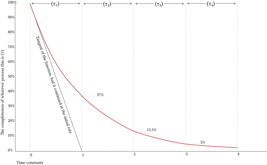
If, instead of curving exponentially and slowing its rate of decay, the function continued to decay at the same rate as it had at Time Zero, it would obviously reach the bottom rather quickly. The time it would take to reach the bottom is one time constant. Because this happens to be an exponential curve (using the base of natural logarithms, e), after one time constant the function has decreased to 37% of its initial value (i.e. it has decreased by 63%). Thus, one might say that the time constant is

“A time which represents the speed with which a particular system can respond to change, typically equal to the time taken for a specified parameter to vary by a factor of 1− 1/ e “

Concept:

• The time constant is defined as the measure of time required for certain changes in voltages and currents in RC and RL circuits.
• The elapsed time exceeds five-time constants (5τ) after switching has occurred, the currents and voltages have reached their final value, which is also called steady-state response
• A Pulse is a voltage or current that changes from one level to another and back again. If a waveform’s high time equals its low time it is called a square wave. The length of each cycle of a pulse is its period 
• A short time constant is defined as no more than one-fifth the pulse width, in time, for the applied voltage.

Example 1: Imagine you have a toy car that can go faster or slower when you press a button. The time constant is like how quickly the toy car gets to the right speed after you press the button. If it takes a long time, it’s slow. If it happens quickly, it’s fast. So, time constant tells us how fast or slow something happens in a special way! 🚗⏱️

Example 2: Imagine you have a magic potion that you use to grow a plant. The time constant is like how quickly the plant grows after you pour the potion on it. If it takes a long time, the plant grows slowly, and if it happens quickly, the plant grows fast. So, the time constant helps us understand how fast or slow things change or develop in a special way! 🌱⏱️

Example 3: Imagine you have a smart home with a thermostat that adjusts the room temperature. The time constant is like the speed at which the thermostat reaches the desired temperature after you change it. If it takes a long time, the temperature changes slowly, and if it happens quickly, the temperature changes fast. So, the time constant gives you an idea of how responsive the system is to changes, whether it’s in a technical circuit or any other dynamic system! 🏠🌡️⏱️

Example 4: When you have a dynamic system, like an electronic circuit or a chemical reaction, the time constant measures how quickly it responds to changes. It’s like a special “reaction speed” parameter. For instance, in an RC circuit, it’s determined by multiplying the resistance and capacitance values. A larger time constant means the system responds slowly to changes, and a smaller time constant means it reacts quickly. Understanding the time constant helps engineers and scientists predict and control how systems behave in real-world situations. 📊⏱️🔌

Example 5: The time constant is a significant concept used in physics and engineering to analyze dynamic systems. It represents the time it takes for a system to reach approximately 63.2% of its final or steady-state value after a sudden change in input.

In various applications, such as electrical circuits, mechanical systems, and chemical processes, understanding the time constant is essential for predicting the system’s response to changes and disturbances. A higher time constant implies a slower response, while a lower time constant indicates a quicker response.

By knowing the time constant, engineers and scientists can optimize and control system behavior, ensuring stability and efficiency in a wide range of real-world situations. 🕰️⏱️🔌🚀

The defining properties of any LTI system are linearity and time invariance.

• Linearity means that the relationship between the input x(t) and the output y(t), both being regarded as functions, is a linear mapping: If a is a constant then the system output to ax(t)is ay(t); if x′(t) is a further input with system output y′(t)then the output of the system to x(t)+x′(t) is y(t)+y′(t), this applying for all choices of a,x(t), x′(t). The latter condition is often referred to as the superposition principle.
• Time invariance means that whether we apply an input to the system now or T seconds from now, the output will be identical except for a time delay of Tseconds. That is, if the output due to input x(t) is y(t), then the output due to input x(t−T) is y(t−T). Hence, the system is time invariant because the output does not depend on the particular time the input is applied.

Physically, the time constant represents the elapsed time required for the system response to decay to zero if the system had continued to decay at the initial rate, because of the progressive change in the rate of decay the response will have actually decreased in value to 1 /e ≈ 36.8%in this time (say from a step decrease). In an increasing system, the time constant is the time for the system’s step response to reach 1 − 1 /e ≈ 63.2%of its final (asymptotic) value (say from a step increase). In radioactive decay the time constant is related to the decay constant (λ), and it represents both the mean lifetime of a decaying system (such as an atom) before it decays, or the time it takes for all but 36.8% of the atoms to decay. For this reason, the time constant is longer than the half-life, which is the time for only 50% of the atoms to decay.

The Time Constant of the lung (TC) is a concept borrowed from electrical engineering (as explained above) which describes the phenomenon whereby a given percentage of a passively exhaled breath of air will require a constant amount of time to be exhaled regardless of the starting volume given constant lung mechanics. That’s quite a mouth-full of a definition but consider what determines how long it takes to exhale a tidal breath passively. At the start of exhalation, the initial flow of gas out of the lung depends upon the driving pressure (i.e. alveolar pressure – mouth pressure) and it depends on the airway resistance. For any given volume of gas, the alveolar pressure at the start of exhalation is only dependent upon the lung compliance. Mathematically, the time constant is defined as compliance multiplied by the airway resistance and the resulting value has units of seconds of time.

• Time constant (τ) is the time required for inflation up to 63% of the final volume, or deflation by 63% 
• It is the product of resistance and compliance
• For a normal set of lungs as a whole, the time constant is 0.1-0.2 seconds

The time constant determines the length of time needed for a passive exhalation and that the time constant is the product of airway resistance and lung compliance. The lower the compliance, the higher the driving pressure pushing gas out of the lungs during exhalation; the lower the resistance, the higher the expiratory flow rate can be when driven by the alveolar pressure. If the time constant is known (or can be estimated) then the maximum mechanical respiratory rate that can be used before Auto PEEP results can be estimated. Consider that at least 3 time constants are required to exhale passively any volume of gas. The combination of inspiratory and expiratory time leads to a give respiratory rate such that:

Total Breath Time = Insp time + Exp time

Respiratory Rate = 60 / Total Breath Time

Maximum Rate = 60 / (Insp time + 3 x TC)

A patient with a compliance of 0.05 L/cm H20 and an airway resistance of 30 cm H20/L/sec. This would give a time constant of 1.5 seconds. A complete exhalation would take around 4.5 seconds. If inspiratory time is 1 second then total breath time is 5.5 seconds and the maximum respiratory rate without gas trapping would be 11 breaths per minute. When gas trapping occurs, the functional residual capacity (FRC) is increased. As the FRC increases, the alveolar pressure increases by an amount of pressure determined by the patient’s lung compliance. As the FRC rises in relation to the total lung capacity (TLC), the lung compliance will decrease. This decrease in lung compliance shortens the time constant for the next breath and thus shortens the time required to exhale the next breath and lessens the amount of trapping that will occur with each subsequent breath until the time constant shortens enough that gas trapping no longer occurs. When this steady state is reached, the FRC is at its maximum and the auto-PEEP is also at its maximum. This fact gives us a way to measure how much auto-PEEP exists since we can serially measure exhaled tidal volumes and then interrupt ventilation (by turning the respiratory rate to zero for several seconds) and measuring how much gas the patient exhales as the patient exhales back to the FRC level that existed prior to ventilation. If we take the difference between the exhaled volume during ventilation and the exhaled volume after interrupting ventilation then we have the amount of gas that was trapped. If we divide this volume by the lung compliance we will have calculated the amount of auto-PEEP applied to the alveoli during ventilation. Normally we are more interested in avoiding auto-PEEP than in measuring it though there are many patients in whom it cannot be avoided so it is useful to be able to quantitate it. Another way to detect auto-PEEP is to watch a patient’s chest movement and/or breath sounds during exhalation to see if exhalation stops prior to initiation of inspiration by the ventilator. If exhalation doesn’t finish then auto-PEEP is occurring. When exhaled tidal volumes cannot be measured (which is seldom with modern ventilators) the level of auto-PEEP can be very roughly estimated by interrupting exhalation just prior to initiation of inspiration and watching to see if there is a pressure increase at the airway as exhalation continues into the circuit between the patient and the point of your interruption. This is not an accurate measurement since the interruption necessarily cuts exhalation shorter than it would normally be and because the circuit volume dampens the pressure measurement but this technique can be useful if you are unable to use the more reliable methods outlined above.

In the presence of constant flow,

• Poor compliance units will have a shortened or normal time constant, and will fill rapidly but incompletely
• High resistance units will have a long time constant, and will fill slowly 
• When flow ceases, gas may flow from lung units with poor compliance into lung units with high resistance
• Exchange of gas between lung units with different time constants is called pendelluft

This has implications for dynamic compliance:

• With decreased inspiratory time, the fraction of the tidal volume delivered to lung units with long time constants will decrease (i.e. all the tidal volume will go to “faster” lung units)
• This will have the effect of decreasing dynamic compliance
• In addition to airway resistance, this factor contibutes to the frequency dependence of dynamic compliance (i.e. dynamic compliance becomes lower with increasing respiratory rates)

For normal lungs, the value for an expiratory time constant is usually given as approximately 100-200 millseconds, i.e over 0.6 seconds 95% of the total lung volume should be emptied. Obviously in states of extreme ICU-level illness, thing may be a little different; especially where airway resistance is increased. For example, Karagiannidis et al (2018) demonstrated time constants around 2500 milliseconds in patients intubated for severe COPD. Interestingly, in ARDS patients, Guttman et al (1995) found expiratory time constants in the range of 600-700 milliseconds, but these were mainly due to the mechanical properties of the endotracheal tube (and the lung itself was not to blame), which supports the concept of a normal but small “baby lung” in ARDS.

Basically, the implication of all these diagrams are that lung units with different time constants will fill at different rates and potentially also up to different final volumes. Then, when the inspiratory flow stops, the lung units with longer time constants (usually described as “slow alveoli”) will continue to fill with “borrowed” gas which redistributes from faster alveoli. This exchange of gas is usually given the term pendelluft, which seems to be the go-to German word to describe any gas movement between different lung units. 

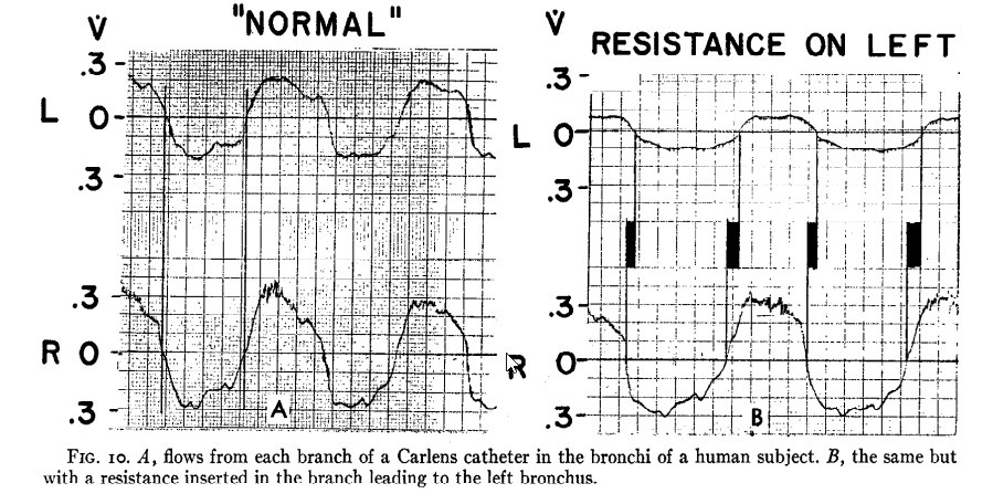
Practically, this can be demonstrated by performing an inspiratory hold manoeuvre on a mechanical ventilator. When one’s mechanical breath has been delivered and the flow stops, the airway pressure first falls abruptly because resistance no longer contributes to it. That part is irrelevant. Then, as one holds the pause for longer, one may be able to see a gradual downward drift of the plateau pressure, as gas is exchanged between lung units with different time constants. This pendellufting of the tidal volume is one of the reasons the recommended duration of an inspiratory hold is about 2 seconds (the other reason for this phenomenon is the relaxation of the lung and chest wall tissues, which contributes to the total airway resistanceand is discussed elsewhere).But how much pendelluftis there in a normal respiratory system? Probably very little. Otis et al (1956) measured time constants from each of the main bronchi belonging to a Dr. Bruce Armstrong, according to the footnote. As one can see from their data (below), “flows in the two bronchi were roughly equal and exactly in phase with each other”. Only when some added resistance was introduced was there a change in the flow timing, seen in the diagram on the right.

Something very similar was the result of some experiments by Bates et al (1988), although these investigators used mongrel dogs instead of healthy colleagues. Alveolar pressure was measured, rather than bronchial pressure, making this somewhat more convincing. There was minimal difference in expiratory flow rates between different lung units in these animals, prompting the authors to remark that “the lungs of these animals …behaved as if they contained a single large and uniform alveolus, with no regional differences in time constants of emptying”.

In summary, in the presence of constant flow,

• Poor compliance units will have a shortened or normal time constant, and will fill rapidly but incompletely
• High resistance units will have a long time constant, and will fill slowly 
• When flow ceases, gas may flow from lung units with poor compliance into lung units with high resistance